
Given the current state of the industry-standard simulation tools, it is possible to reduce the development time of new products by 50% or more by employing software-in-the-loop (SIL) technologies in the design process. That is if you have the right model to simulate. What are the varying levels of complexity in vehicle modeling, which model to use, and how to use them? Let’s find out.
What is it for?
A vehicle model, in essence, is the mathematical representation of a vehicle and is a powerful asset to any automotive engineer’s work in understanding how a vehicle behaves under changing operating conditions, and how it responds to certain modifications and developing tools. A vehicle model can be employed in several roles in the development process of any product.
- Simulation: A model with an adequate level of fidelity can be used in simulation to test out in-development components, software, control algorithms, and even whole new vehicles and save precious testing time. It also cuts down the need for hardware-in-loop (HIL) testing which significantly reduces the cost of prototyping.
- Performance & Safety Analysis: Thanks to modern simulation software, availability of key metrics, and data tools, it is possible to assess the performance and safety of new products even before they hit the prototype phase.
- System Integration: A simulation model can be used to test the integration of multiple components or control algorithms and assess their interactions when they cooperate on the same system.
- Digital Twin: By employing a digital twin of a real-world system, wear conditions and possible faults can be predicted ahead of time opening the way for predictive maintenance and fault detection applications. Also, by employing a digital twin, it is possible to produce synthetic data for machine learning and AI development. You can read more about digital twins and AI in our recent post here.
- Model-Based-Control (MBC): Internal models constitute the backbone of certain control methods like optimal control and predictive control. In general, these methods use an internal model of the target plant to plan ahead an optimized control strategy with respect to a performance (or cost) function and a set of constraints.
All these use cases raise their own concerns and limitations. For example, the increased complexity of the model is always undesirable from the perspective of computational power and time optimization, but it generally is just that, an undesirable outcome. However, it becomes a hard limitation, for example, when an online predictive controller on a vehicle needs to simulate the internal model multiple times within a predetermined sampling time with the computational power available to the control unit.
Kinematics Modeling
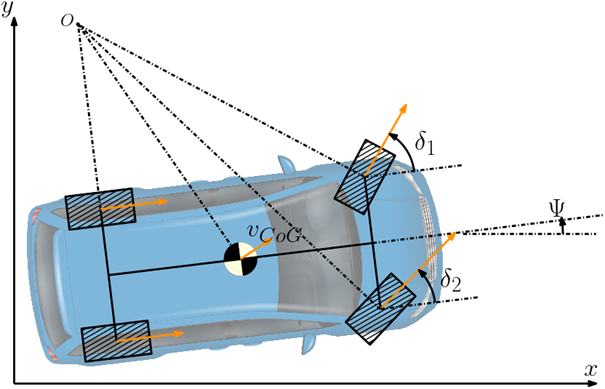
The simplest form of modeling employed for vehicles is the kinematics model where the forces acting on the vehicle body are disregarded, and the motion is considered in a purely geometrical sense. The following conditions should be satisfied for this approach to succeed:
- Out-of-plane motions like roll and pitch are limited or negligible
- Contact between the wheels and the road surface is firm enough to assume non-slip conditions
- Vehicle bodies are sufficiently rigid
These conditions are mostly met while considering low-speed maneuvers in non-extreme road conditions which makes the kinematic modeling approach a very common choice for low-speed applications like parking, docking, and indoor applications.
The states used in the kinematics equations typically contain:
- 𝑥,𝑦 : Planar coordinates of the vehicle center of gravity
- Ψ : The heading angle of the vehicle
- 𝛿 : Steering angle, ususally considered as the input
Kinematics models for ground vehicles have been successfully used for control applications including feedback linearization, motion planning in unobstructed spaces, path following, path planning/following in constrained spaces.
Dynamics Modeling
Relying on purely kinematics models for the vehicle may swiftly become infeasible while considering realistic driving conditions because the assumptions suggested for the kinematics model are only valid under very ideal conditions. In situations where the vehicle operates at a larger speed range, the tire-road contact is hindered (due to weather conditions, tire wear, and off-road applications), extreme maneuvers are required, and the kinematics models become insufficient. As a result, force balances on the vehicle bodies need to be addressed.
The external forces on a typical vehicle include tire forces, gravitational body forces, and aerodynamic forces. There are several ways to commonly address and simplify these forces. These forces are commonly modeled to be determined by other vehicle states to reduce the complexity and dimensionality of the overall vehicle model. For example, the aerodynamic force is usually assumed to depend on the power of the longitudinal speed using a constant aerodynamic coefficient. That is why in the models below, aerodynamic force doesn’t appear explicitly.
Another important point to make here is the determination of the lateral tire forces. Although it is not the focus of this text to discuss the different tire models with varying degrees of complexity and accuracy, their existence should at least be acknowledged. Modeling of the lateral tire force is a crucial part of vehicle modeling, however, commonly, the models are set up such that the lateral force is determined completely by the other states and inputs of the vehicle model. For example, one of the simplest ways to model these forces is the linear cornering force model, where the lateral force acting on the tire varies linearly with the side slip angle of the wheel which is the difference between the heading direction of the wheel vs. the velocity of the wheel. Since this side slip angle can be determined by the vehicle slip angle, steering angle, and the vehicle geometry, the tire force in this case is dependent on the vehicle states and thus not presented as an explicit state. Other popular approaches to tire modeling for this purpose include the magic formula by Pacejka and various combined steering and braking models.
With that, some of the common vehicle dynamic modeling approaches can be summarized as follows.
Single Track (Bicycle) model
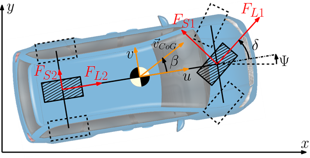
The simplest commonly used approach to dynamics modeling is the bicycle model, where the left and right wheels on the same axle are considered as a lumped unit along the center-line of the vehicle body. This model neglects the load and the reactive force variations between the left and the right wheels and provides a simple set of force balances and dynamics which is especially favorable from a controller design point of view.
Typically, the states and inputs considered in the bicycle model include:
- 𝑢 : Vehicle longitudinal velocity
- 𝑣/𝛽 : Vehicle lateral velocity or vehicle side slip angle are used interchangeably
- ψ, ψ.: Yaw angle and yaw rate, determine the heading angle and its rate of change
- 𝛿 : Steering angle, usually considered as one of the inputs
- FL1,FL2 : Longitudinal tire forces, usually considered as the tractive/braking input(s)
This model neglects out-of-plane motions like roll and pitch, also it cannot account for the effects of uneven road contact, load distribution/shifting, and yaw moments caused by uneven tire force distributions. Therefore, the model is a great choice for small vehicles under common driving conditions (urban speeds, normal road conditions, no extreme maneuvers, etc.) or any size vehicle in low-speed path planning applications like parking, constrained space navigations, and so on. The bicycle model has been successfully employed in vehicle control research on topics including parameter estimation, actuator fault detection, and obstacle avoidance path planning.
Double Track model
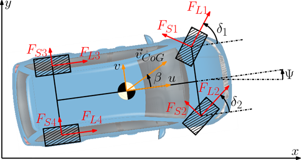
The more commonly used method for dynamics modeling of vehicles considering a larger extent of operating conditions is the double track model. Here, the tire forces are not lumped and treated as separate forces on each side of the vehicle. Thus, the model can account for the yaw moment generated by the offset of the tractive/braking forces on each wheel from the center of gravity. This type of modeling allows for, most notably, yaw stability control via differential braking and torque vectoring.
Commonly, the states and inputs considered in the double track model include:
- 𝑢 : Vehicle longitudinal velocity
- 𝑣/𝛽 : Vehicle lateral velocity or vehicle side slip angle are used interchangeably
- ψ, ψ.: Yaw angle and yaw rate, determine the heading angle and its rate of change
- 𝛿1,𝛿2 : Steering angle of the left and right wheels, usually considered as inputs
- FL1,FL2,FL3,FL4 : Longitudinal tire forces, usually considered as the tractive/braking input(s)
This model neglects out-of-plane motions like roll and pitch, also it cannot account for the effects of uneven road contact, load distribution/shifting, and yaw moments caused by uneven tire force distributions. Therefore, the model is a great choice for small vehicles under common driving conditions (urban speeds, normal road conditions, no extreme maneuvers, etc.) or any size vehicle in low-speed path planning applications like parking, constrained space navigations, and so on. The bicycle model has been successfully employed in vehicle control research on topics including parameter estimation, actuator fault detection, and obstacle avoidance path planning.
Yaw-Roll-(Pitch) Models
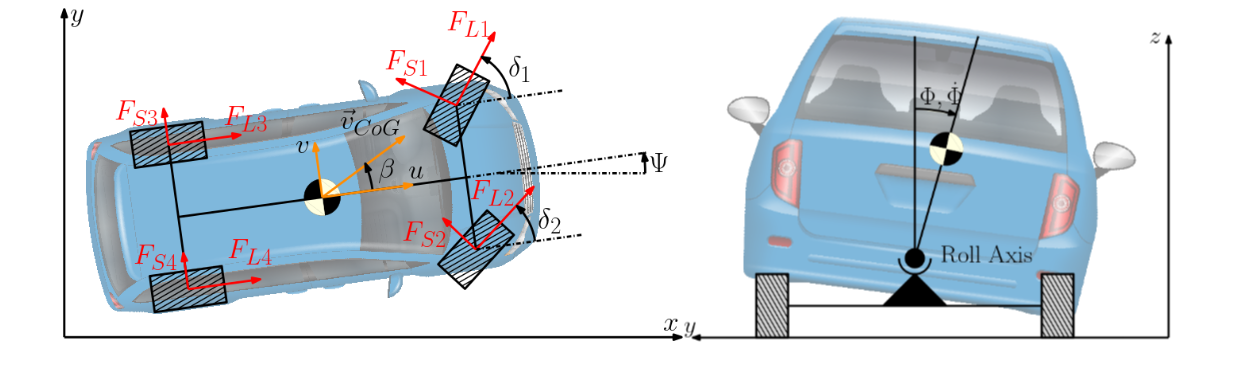
The velocities that necessitate the use of a double-track model also raise concerns for out-of-plane motions, especially in large trucks, buses, and articulated vehicles. Since these vehicles tend to be long and have higher centers of gravity, the side forces generated by the tires and disturbance effects like side winds create a significant rolling moment. If not addressed, this rolling moment, in extreme cases, can lead to load shifting between the left and right sides of the vehicle, causing insufficient road contact on one side of the vehicle and eventually a complete rollover of the vehicle. The yaw-roll and pitch-yaw-roll models are successfully employed for such scenarios. These models typically consider a double track model for the planar motion coupled with the out-of-plane dynamics for pitch and roll motions.
Most commonly, the states and inputs considered in the yaw-roll and pitch-yaw-roll models include:
- 𝑢 : Vehicle longitudinal velocity
- 𝑣/𝛽 : Vehicle lateral velocity or vehicle side slip angle are used interchangeably
- ψ, ψ.: Yaw angle and yaw rate, determine the heading angle and its rate of change
- φ, φ.:Roll angle and roll rate
- θ, θ.: Pitch angle and pitch rate
- 𝛿1,𝛿2 : Steering angle of the left and right wheels, usually considered as inputs
- FL1,FL2,FL3,FL4 : Longitudinal tire forces, usually considered as the tractive/braking input(s)
Typically, in roll and pitch models, the vehicle body consists of two connected masses; sprung and unsprung mass. The out-of-plane motion of the unsprung mass is usually neglected. The sprung mass is usually free to rotate around a so-called roll axis. The roll axis is usually fixed with respect to the unsprung mass or in some models it can rotate with the pitch angle of the vehicle. Since this rotation of the sprung mass is around an off-center roll axis, it changes the load distribution of the vehicle and available frictive forces between the wheels on the left and right sides of the vehicle. In extreme situations, this load shifting can completely negate the road contact on one side of the vehicle which is referred to as a rollover.
The pitch motion of the vehicle is usually due to strong braking or accelerating and in most cases negligible. Like the rolling motion, the pitch angle of the sprung mass creates a load shifting from the rear to the front or vice versa. This load shifting, again, results in a change in available frictive force in the front and rear tires and is a serious concern with high-performance vehicles like racing cars and tall vehicles with a short base like tractors.
Special Case: Articulated Vehicles and Trailer Systems
When vehicle articulation is considered, the most common approach is to assume any of the kinematics or dynamics models described above and define them separately for each tractor and trailer. The main issue arises from the contact point between each vehicle body, commonly referred to as the hitch point. For the contact at the hitch point to remain intact in the mathematical model, a number of constraint equations are needed. These equations may be obtained by setting the kinematics of the hitch point to be equal from the perspective of both connected bodies. For example, in the case of a dynamics model, this approach can be used to calculate contact forces generated at the hitch point.
Interested?
At Combine, with our expertise in the automotive industry, we can help build your vehicle models and tailor them to your needs.
Read more about digital twins and AI in our recent post here.